
Simple linear regression
assume a model : (Y≈β_0+β_1X)
β ̂0intercept β ̂1 slope Given some estimates β ̂0 and β ̂1, we can predict future sales y ̂=β ̂0+β ̂1x
regression: continous variable> grwoth of crop(soil,country) classification: discrete
Estimation of the coefficients
- the prediction for Y based on the ith value of X. (yi) ̂=β ̂0+β ̂1xi
- ==residual== 残差 ei=y_i−(yi) ̂
- We define the ==residual sum of squares (RSS) ==as RSS =e_1^2+e_2^2+…+e_n^2 RSS =(y1−β ̂0 −β ̂1x1)2+(y2−β ̂0 −β ̂1x2)2 +…+(yn−β ̂0 −β ̂1xn)2
- Mean squared error: MSE=1/nRSS
- ==计算题==minimize the function: The least squares approach»minimize the residual sum of squares β ̂0 and β ̂1 such that the RSS is minimized. best possible line β ̂1=∑_i=1^n sum(x_i−x ̅)(y_i−y ̅)/∑_i=1^n sum(xi−x ̅)2 , β ̂0= y ̅−β ̂1x ̅, where y ̅=1/n∑_i=1^n sum yi and x ̅=1/n∑_i=1^n sum xi are the sample means. ==证明题== Exercise 6: Using, argue that in the case of simple linear regression, the least squares line always passes through the point mean x and mean y
The residual standard error
- The approximate relationship: Y=β_0+β_1X+ε, Where ε is a mean-zero random error.
- The better the fit, the smaller the standard deviation of ε σ =std (ε)= √RSS/(n−2)= ==RSE (the residual standard error)== 残差和的标准=残差标准差
- 这个可以再来计算standard errors of the coefficients(SE(β ̂0) and SE(β ̂1))去确定这个prediction interval(预测区间=预测值±tα/2×预测标准误差)
- 或者去计算confidence interval :β ̂1±2∙SE(β ̂1)
- 最后 A 95% chance that the interval contains the true value of β1. [β ̂1−2∙SE(β ̂1), β ̂1+2∙SE(β ̂1)]
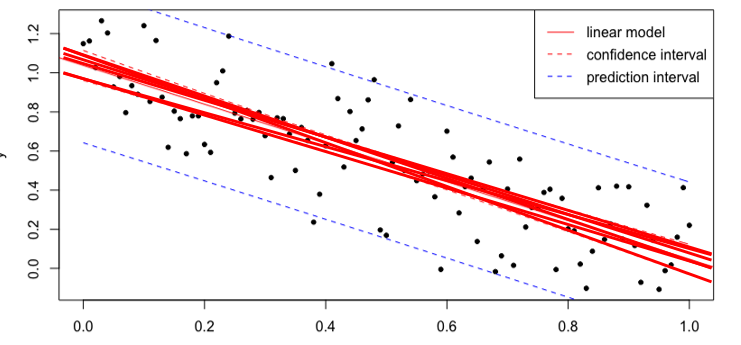
Model Uncertainty
Confidence Interval
置信区间用于估计==参数==的不确定性范围
Prediction Interval
预测区间用于估计未来==观测值==的不确定性范围。
Hypothesis testing
- 描述 H_0:There is no relationship between X and Y versus the alternative hypothesis H_1: There is some relationship between X and Y
- 在数学上表示就是: H_0 : B1 = 0 就是slope=0 H_1 : B1 != 0 就是slope !=0
- to test the null-hypothesis, we use ==t- statistic== t=β ̂1−0/SE(β ̂1)
- p-value gives the probability of the null-hypothesis being true ==if p <0.05, the 零假设 not likely to be true, so X 和Y has relationship==
- Assuming β1=0 (H_0), t follows a t-distribution with n−2 dof 当我们测试 β1=0 这个假设时,我们计算得到一个 t 统计量,其分布遵循 t 分布,自由度为n−2。这个 t 统计量告诉我们在 β1=0 假设成立的情况下,我们观察到的数据有多不寻常。
- t- distribution: 它类似于标准正态分布,但是它的尾部更加厚重,这使得 t 分布更适合于小样本情况下的推断
- 自由度: t 分布中的一个参数,它决定了 t 分布的形状
Assessing the accuracy of the model
- RSE 越小越好
- RSS
- R-squared = 1- RSS/TSS (0-1) 越大越好 RSS=∑_i=1^n sum (yi−y ̂i)2 is the residual sum of squares TSS=∑_i=1^n sum (yi−y ̅)2 is the total sum of squares
- R2 statistic vs correlation(r)
- R²仍然是用来衡量模型对因变量的变异性解释程度的指标
- r相关系数通常用来衡量每个自变量与因变量之间的线性关系>r^2是加权平方和
- 当p=1(only has one X ): R^2=r^2 (only for simple linear regression, p=1)
Analysis
- The ==Residual standard error ==is a rough estimate for the standard deviation of ε, so, the standard deviation of the model prediction error. So in our advertisement example, the model will predict on average with an accuracy of 3.26 (thousand) sold units.==多少个== - The ==R2== value indicates that 61.2% of the variance in the data set is explained by the model. ==多少占比== # Multiple linear regression - 公式 - the definition of partial slope: We interpret βj as the average effect on Y of a one unit increase in Xj, holding all other predictors fixed. - two predictors (p= 2变量)> 3D - more predictors(p > 2)> hyperplane in p-D space - 但是还想最小化这个点到面的距离,就是minimize RSS ## Correlation between regressors - confounding variable 当单独TV,newspaper的时候,p value both < 0.05, but when taking TV, newspaper and radio as the X variables together, the p value of newspaper >0.05,因为newspaper 和radio相关,in other word, newspaper is confounding variable(混交变量) ## 1.Relationship between response and predictors ### F- statistic 就是跟t-statistic一样的 #### F=((TSS−RSS)/p)/(RSS/(n−p−1)) - F is high when ==RSS== is low Better fitting model, higher F - F compensates for number of independent variables p F lower, when more variables used - F increases with the number of samples n ##### When F-statistic close to 1 , there is no relationship between the reponse and predictors - If the linear model assumptions are correct: E{RSS/(n−p−1)}=σ^2 - If H_0 is true: E{(TSS−RSS)/p}=σ^2 ##### When H_1 is true, E{(TSS−RSS)/p}>σ^2, F > 1 ## 2. What are important variables? We would like to select the best predictors - Trying to ==compare all possible combinations== of models requires 2^p models to be built, including parameter estimation. For p=30, this means over a billion models.
- To overcome computational capacity problems, some ==automated selection procedures== have been developed.
Selecting the best model/features
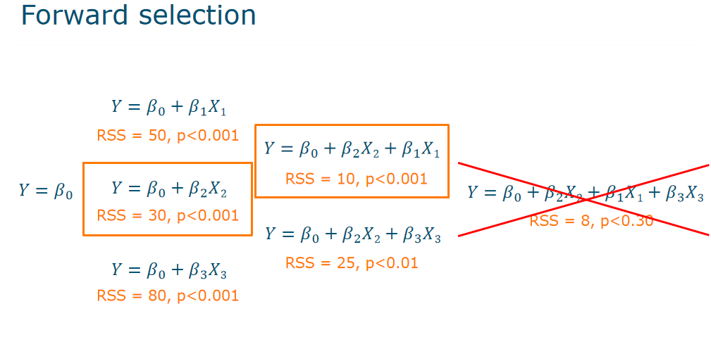
Forward Selection
Begin with the ==null model==: Y=β_0 Try to ==add== one variable: Y=β_0+β_1X1, Y=β_0+β_2X2, Y=β_0+β_3X_3 Pick the one-variable model with ==lowest RSS == ==Repeat== to get best two-variable model ==Stop== when none of the remaining variables have a significant contribution就是当p大于0.05之后
Backward selection
Start with ==all variables== in the mode ==Remove variable== with ==the largest p-value== Fit new ==(p-1)-variable model== Remove ==next variable with largest p-value ==to get to (p-2)-variable ==Continue== until ==stopping rule== (largest p < threshold)
Mixed
3. How well does the model fit the data?
- R^2: <mark class="hltr-grey">Portion</mark> of explained variance in the data Adding more variables will never reduce R2 - RSE(Residual Standard Error): RSE≈ standard deviation of ε more parameters mean higher p which contribute to an increasing RSE ## 4.How accurate are the predictions? Three causes of prediction uncertainty - ==The accuracy with which the βi can be estimated.== This is related to the <mark class="hltr-grey">reducible error</mark>, and is dependent on the type and amount of data - ==The inherent model error. ==Not all processes are linear, so if we decide to choose a too simple model, there is <mark class="hltr-grey">model bias.</mark> - ==The random error, ==modelled by ε. For each new experiment, some random error can be involved due to measurement noise, or some other unexplained variance source. This is the<mark class="hltr-grey"> irreducible error. </mark> # Extension of the linear regression ## Qualitative predictors定性 #### dummy variables 虚拟变量来数学表示qualitative predictors 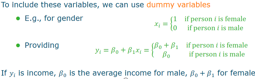 #### Dummy variables for more than two levels 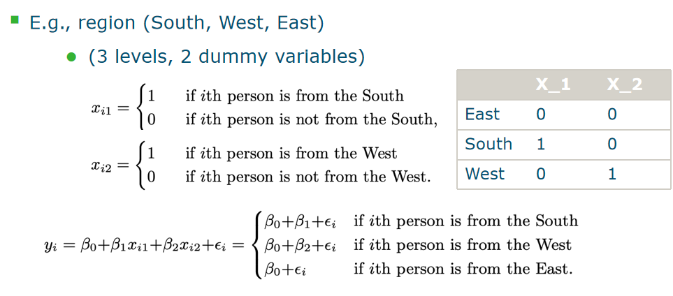 ## Interaction Terms #### Assumptions of linear regression model: - ==Additive:== the influence of Xj on Y is independent of other variables - ==Linear:== doubling the size of Xj will double its effect on Y. #### extra interaction Y=β_0+β_1X1+β_2X2X3+ε. This model is not additive anymore, and ==nonlinear ==in the variables. However, it is still linear in the coefficients. 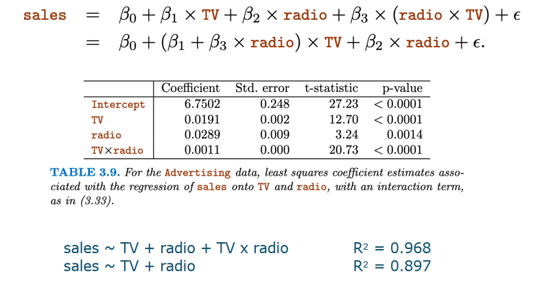 ## Polynomial Regression/cubic Nonlinear relationships can be modelled by polynomial regression.
Exercise 3 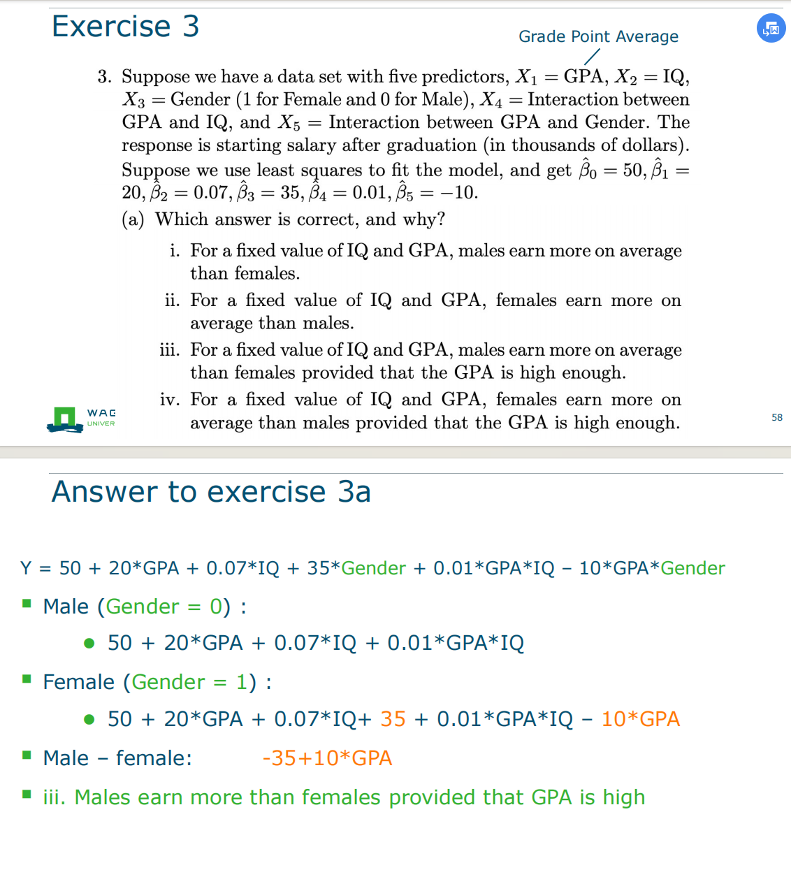
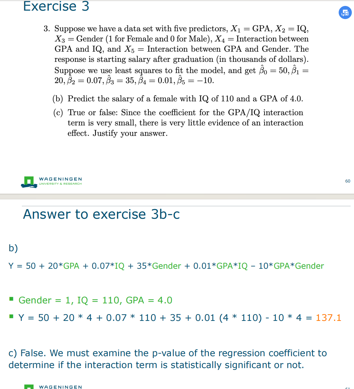 False: Since the ocefficient for the GPA Exercise 4 cubic and linear
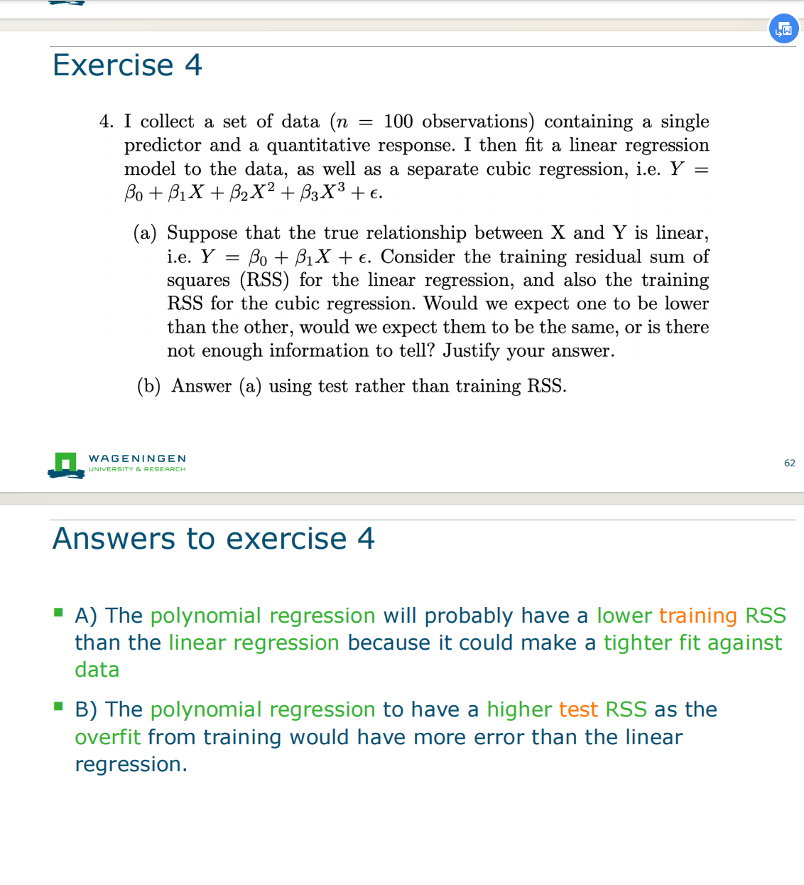
Inspecting data and model可能会出现的问题
1. Nonlinearity非线性
==Residual plots== can be useful to identify nonlinearity of the data 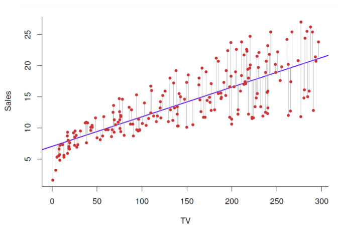
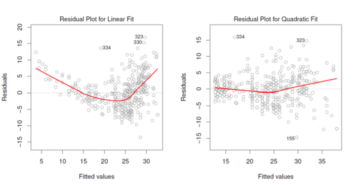 都是和intercept那个线来比较,来求距离。 ==The residuals ==ei=y_i−y ̂_1 of the linear fit (left) show a strong pattern. ==Quadratic fit ==(right) has more equally distributed residuals.
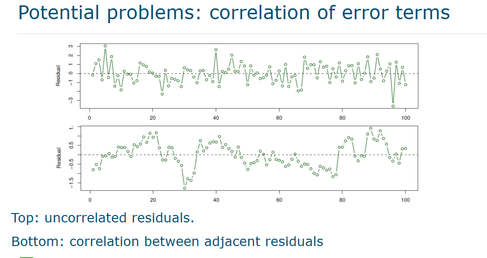
2. Correlation of error terms相关性
- 两个independent variable之间有没有关系
- ==Important assumption==: for each observation j, the ==error terms εj are uncorrelated==. This assumption is not always true.
- In time series data, residuals are often ==correlated==, which causes ==tracking== – adjacent residuals show similar values
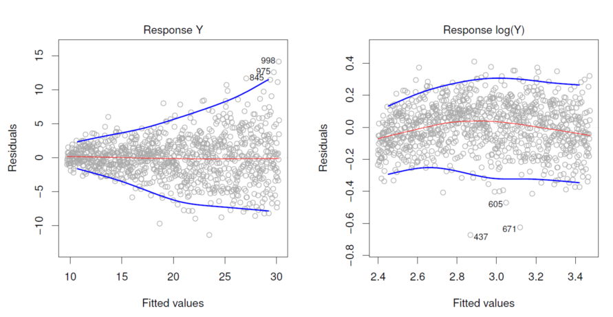
3.Nonconstant error variance: 异方差性
- Important assumption: constant variance Var(εi)=σ2 for all i.
- This does not always hold true :heteroscedasticity
- A possible way to ==solve== this is by transformation of Y such as log(Y) or √Y
4. Outliers离群值
- ==Outliers==: points yi that are far from the value predicted by the model
- ==Possible caused==: incorrect measurements or recordings
- Outliers may ==cause ==RSE to increase, and R2 to decrease
- Check for outliers visually: via residual plots
- ==Studentized residual==: t_i=ϵ_i/SE(ϵ_i)学生残差的计算方式是将残差除以一个标准误差的估计量,通常使用的标准误差是根据样本数据得到的回归模型的残差标准差.==就是另一种除法的标准残差==
- Test statistically on outlier: |t_i|>3
5.High leverage points高杠杆点
- High leverage points: ==unusual high or low x values== > have much influence on estimated values of the coefficients
- Leverage stats: ℎ_i=1/n+(x_i−x ̅)^2/∑_j=1^n▒(x_j−x ̅)^2
- Average leverage =p+1/n
- If ℎ_i≫p+1/n , a point is a ==high leverage point. ==
6.Colinearity/corelation
- ==Collinearity==: two or more predictors are closely related to each other
- This may ==cause== high uncertainty in coefficient estimates
Measuring collinearity: ==Variance Inflation Factor (VIF) ==
VIF(βj)=1/1−R_X_j X_−j^2大代表相关性高 with R_X_j X_−j^2 the R2 from a ==regression of Xj onto all other predictors.== - VIF is high when X_j can be estimated well from other variables
- ==VIF(βj)>5 or 10== is indicates problematic amount of collinearity
- Action: remove predictor with largest VIF and perform analysis again for the simpler model
- ==VIF high, it can be moved one of them maybe==
文档信息
- 本文作者:Xinyi He
- 本文链接:https://buliangzhang24.github.io/2024/02/03/MachineLearning-2.-Linear-Regression/
- 版权声明:自由转载-非商用-非衍生-保持署名(创意共享3.0许可证)