KNN,LDA and QDA are Bayesian classification

Classification

Finding class k that maximizing the conditional probability 举例来说，如果你的任务是将一张图片分类为狗、猫、或鸟，那么你可能会得到每个类别的概率，比如：

• 狗：0.8
• 猫：0.1
• 鸟：0.05 在这种情况下，P最大化的类别是狗，因为它有最高的概率。

  K-nearest neighbor classifier

  ![[3e88de363372e84e89e86b1b6e3e538.png]]

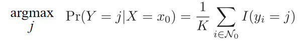
• non-parametric
• what probability the point belongs to the class j,as the fraction of points in ==N_0== whose reponse values equal ==j==
• N_0 contains the ==K== points that are closest to x_0

  Example

  ![[8901136cb31a6453aa079dee0193561.png]]

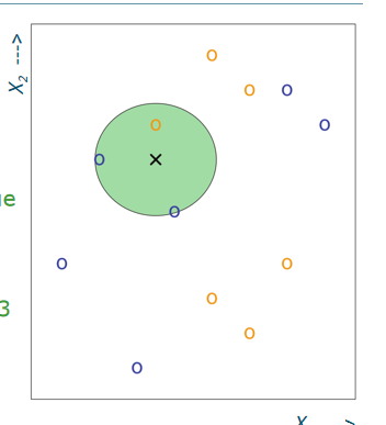
• K= 3 表示有三个最近的点在这个sample 点的附近
• the region of the cricle :the last nearest neighbor
• Size of the green circle varies, depending on the location of the black cross
• x1 10000 but x2 78. the scale , the dominated by x1

  Decision boundary

  ![[f4558634bdc194c0c0d463969e5fa1d.png]]

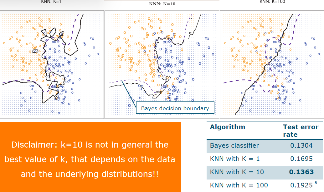
• Corresponding KNN ==decision boundary== P(Y = blue | X) =P(Y = orange | X) = 0.5 if there are three classes，=0.33
• 迭代error, test overfiting on the nosiy
• We have the Bayes Decision boundary automatically

  How to choose K

• K= 1: decision boundary overly flexible high variance ,overfitting
• K=100: decision boundary close to linear high bias underfitting
• K= 10 just right in this case only ==validation set== to choose which K is the best

  Training and test error

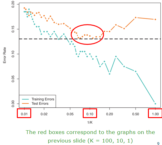  ![[8c4be1a107e87038c7033c72ebe0d80.png]] 1/K related to flexibility of kNN K smaller, 1/K bigger, more flexible

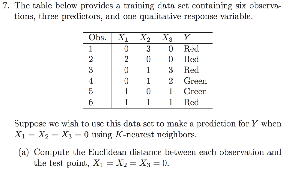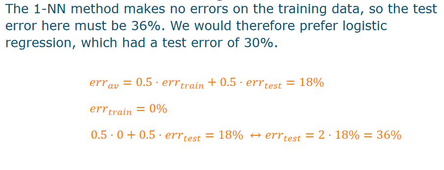
exercise2.7 Compute the Euclidean distance between each observation and the test point X1 = X2 = X3 =0 ![[Pasted image 20240215104122.png]] d(x_i,x_j)=√(X_i1−X_j1)^2+(X_i2−X_j2)^2+(X_i3−X_j3)^2 if K= 1 , bigger than 1 is red if K= 3, bigger than 3 is red exercise 2.8 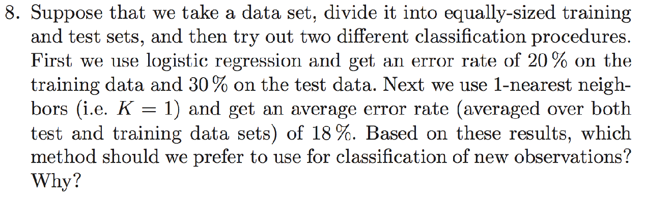![[Pasted image 20240215104552.png]] (在这个问题中，我们有一个数据集，将其分成相等大小的训练集和测试集，然后尝试两种不同的分类方法。首先，我们使用逻辑回归，得到训练数据的错误率为20%，测试数据的错误率为30%。接下来，我们使用1个最近邻方法，得到的平均错误率（在训练和测试数据集上进行平均）为18%。基于这些结果，我们应该更倾向于使用哪种方法来对新的观测进行分类？)

• 鉴于1-最近邻方法在训练数据上没有错误，那么测试数据的错误率必须是36%（1-最近邻测试错误率=18%*2=36%）。在这种情况下，逻辑回归方法更可取，因为它的测试错误率更低，为30%。感谢您发现了这个错误。
• ![[64102d655b447fb1f664ea0742b1f6f.png]]

  Bayesian Classification

  Classification

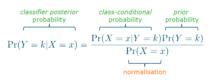
  posterior probability

  Class- conditional probability

  So, Pr(Y=k|X=x) is difficult to model The reverse, Pr(X=x|Y=k), can be estimated easily 第一句话是指对于给定的数据点x，预测它属于类别k的概率是多少，这是一个困难的问题。第二句话则是指给定一个类别k，估计数据点x属于该类别的概率是多少，这通常是一个相对容易的问题。 本来是这个颜色是不是属于苹果，变成了给定一个数据点属于苹果类别，预测它的颜色是什么

  Bayes’ theorem in classification

  ![[26053c986aaef35d67bccec6fb29d5a.png]] ![[dbfeebe5590b7a96acabe5847258a2d.png]]

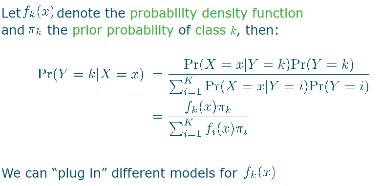
  Bayesian plug-in classifier

  ![[839fbd7e28217691b6ddb0d57c6c326.png]]

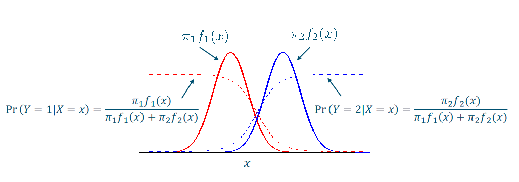
• 实线/ dash line的和是1
• the interaction of dash line is 0.5
• if > dash line , it is class 1 assign class label with highest posterior

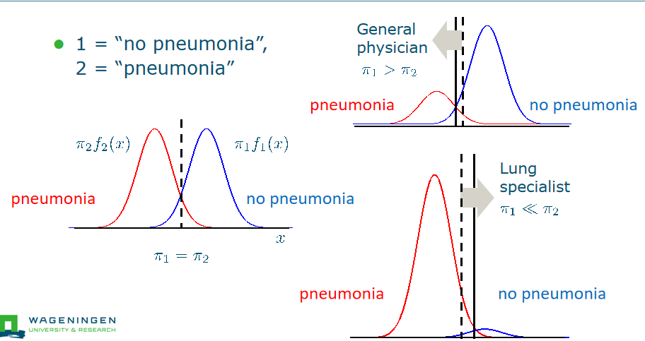
  influence of prior

  ![[077332f8a3a195c4246fe2992b08f70.png]]

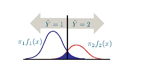
  Bayes’error

  Bayes’ error: theoretically minimum attainable error ![[67311154b7f5446707998dc0e7fee4e.png]]

  Class-conditional distributions

  simple solution: historgrams assume normal(Gaussian) distributions

  Linear Discriminant Analysis

  Normal distributions

  ![[2d07ad72d164b1574d70e6407423197.png]]

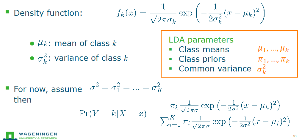
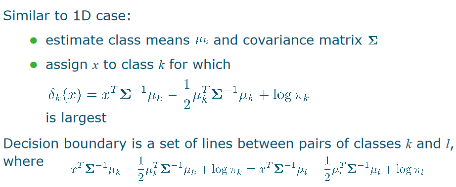
  Linear discriminant analysis(LDA)

  ![[3afae7768aace32d3ff37bd6e4d748c.png]] singma is same shape is same k classes maximize the function too 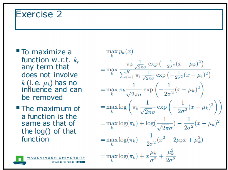![[0442a9a035f3604ca35cd1854ef5b7c.png]] 这个下面这一坨都是indepent of k，因为它对每一个k都是一样的 exercise 7 ![[a4480ec426829397298f17dd0a22835.png]]

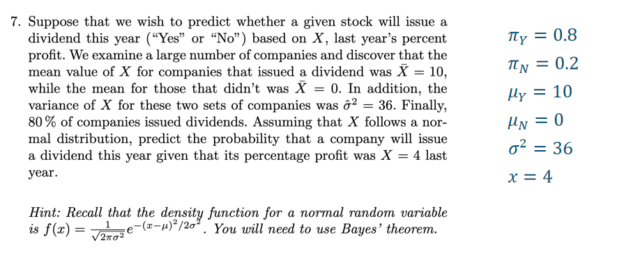
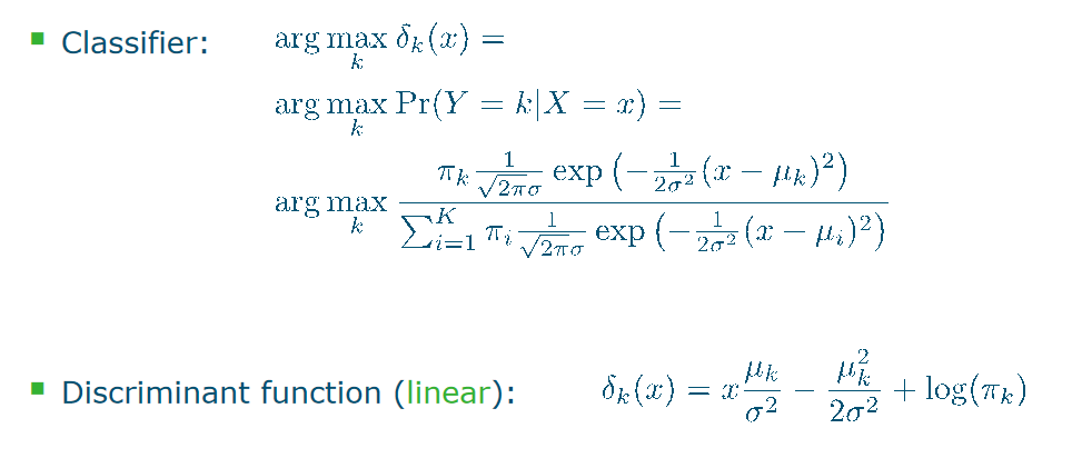
  Nearest mean classifier

• Assume ==priors are equal==, pi1 = pi2 = pi, then decision boundary is at 就是class 1 variance= class 2 variance
• use the Discriminant function: calculate the value of x at the decision boundry : x=(u_1 + u_2)/2 ,so the decison boundary between the two means
• Assign x to class with nearest mean

  Linear discriminant analysis

• 在实践中，我们使用样本均值和样本标准差来估计总体均值和总体标准差，然后使用这些估计值来计算每个类别的观测概率。然后，根据这个概率来做出预测。
• ==就是 u> variance > pi== ![[4fd5f1d7f7f7bc8157a83cc54a84018.png]]n1 the number of the samples
• Assumes dataset is an independent identically distributed (iid) sample of underlying distribution(这意味着数据集中的每个样本都是来自相同的分布，并且每个样本都是相互独立的，没有重叠或重复的样本。)

  parameter estimation

  In general: the more samples, the better the estimates (dashed lines,就是mean， variance 的估计的形状更好) and the better the classifier

  the Multivariate Case

  If p > 1: same classifier, using multivariate Gaussian

  Multivariate LDA

  ![[1a51c6fc1348ad22852dec663fdbb60.png]]

  Quadratic Discriminant Analysis

• ==LDA== assumes each class has the ==same covariance matrix Σ; ==estimated by weighted averaging of per-class covariances Σk
• ==QDA== is the same classifier, with a Gaussian distribution with a ==separate covariance matrix Σk for each individual class==
• Assign x to class k for which the ==(quadratic) discriminant function== is largest. ![[Pasted image 20240218153413.png]]
• for a p-dimensional data set:
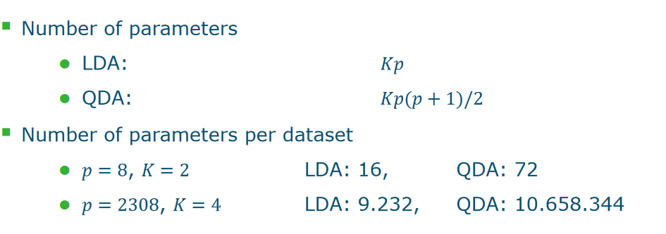
  mean_k: is a vector with ==p elements== covariance_k : is a matrix with ==0.5 p(p+1)== elements
• need more samples
• computational complexity:LDA:==K×p==, QDA:==K×p(p+1)/2 == ![[ed227359b380886b891aefb687c0d7f.png]]

  Curse of Dimensionality

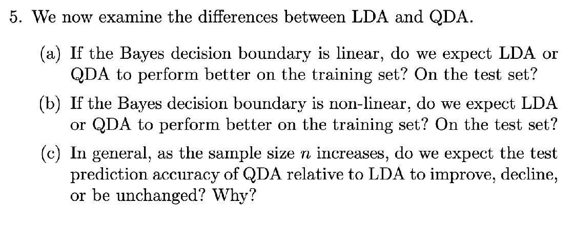
  exercise 5 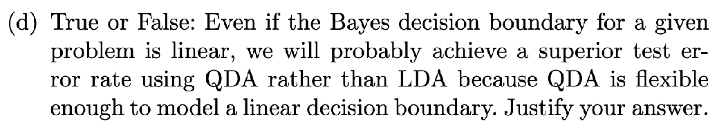![[Pasted image 20240218160053.png]] ![[Pasted image 20240218160058.png]] a) QDA on the training set, LDA on the test set:QDA is likely to overfit here, LDA not. QDA在训练集上表现更好：QDA是一种更灵活的模型，允许每个类别有自己的协方差矩阵。当贝叶斯决策边界是线性的时候，QDA可以更好地拟合训练数据，并且可以有更高的训练精度。==但是在test set 上就QDA可能会过拟合，因为它有更多的参数需要估计。== LDA在测试集上表现更好：相反，LDA假设所有类别的协方差矩阵相同，更倾向于学习一个简单的线性决策边界。这使得LDA更容易泛化到新的数据上，从而在测试集上表现更好。 b) That depends on the exact form of the decision boundary,but in general LDA cannot find nonlinear decision boundaries, so given sufficient training data we expect QDA to do better on both. c) Improve, as there are ==more samples to estimate QDA’s additional parameters.== d) False: the additional parameters (for the flexibility) need to be estimated; as a result, QDA can overfit for limited sample size.

  Concept

  When the number of features p is large, there tends to be a deterioration in the performance of KNN and other local approaches that perform prediction using only observations that are near the test observation for which a prediction must be made. This phenomenon is known as the curse of dimensionality, and it ties into the fact that non-parametric approaches often perform poorly when p is large. 当特征数 p 很大时，KNN 和其他利用邻近观测进行预测的本地方法的性能往往会下降。这种现象被称为维度诅咒，它与非参数方法在 p 很大时往往表现不佳有关。 ![[Pasted image 20240218161437.png]] if very few observations are “near” in feature space(the chances are very small), you will use “far away” neighbours instead ANSWER d) If you want 5 samples in the interval: p=1 => 50 samples p=2 => 500 samples p=3 => 5000 samples … We need exponentially more samples with increasing p

  Performance of the classifier

  Sensitivity vs. specificity

  ![[c03b60aefef546e28f4bc24095f7ac0.png]]

  Threshold of the posterior

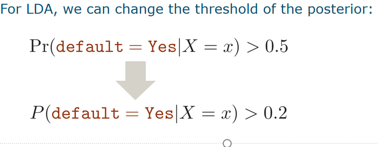
  let us make the LDA classifier more sensitive, allowing the bank to detect more high-risk individuals (==less false negatives==),at the cost of rejecting the credit card applications of some additional low-risk individuals (==false positives==) 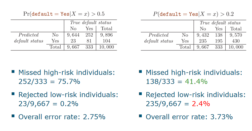![[a1f65370ad40265f4feba4bfe3ccf51.png]] ![[969fd06c50042a81513120ceccd11cf.png]] 就是threshold的值减小，模型更敏感，FN下降，FP上升

  ROC

  ![[fe75ce815df397a4159f5b165794322.png]]

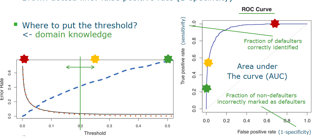
• ROC curve：area is bigger , better
• Black curve: overall error rate
• Blue dashed line: false negative rate (1-sensitivity)
• Brown dotted line: false positive rate (1-specificity)

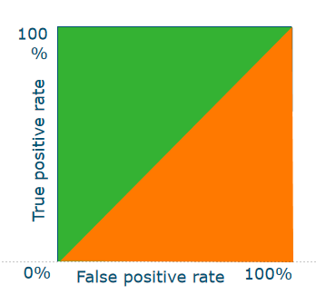
  Area under the curve (AUC)

  If we do not know the optimal operating point (yet), we can summarize the ROC with the area below it: AUC

• optimal: 1
• random classifier: 0.5 ![[5e52b6a919ca434c2ea22a742cedc0a.png]]

  Parametric vs. non-parametric

• ==LDA and QDA are parametric methods==: assume a global model, estimate its parameters
• Non-parametric methods estimate densities locally, which can be an advantage for ==non-linear ==problems and high-dimensional data