supervised learning 的缺点：

• little labelled data available
• generating labels is expensive

  Unsupervised learning

• Discover structure in only X1, X2, …, Xp
• Part of explorative data analysis, very useful in data science
• Main problem: no clear way to check the answer
• Two types of approaches: dimensionality reduction, clustering

  Principal component analysis(PCA)

  find a linear low-dimensional representation that captures as much variation in the data as possible( projection from p dimensions to d < p)

  Dimensionality reduction

• How to investigate high-dimensional data? scatterplots, correlation or covariance, select most interesting

  概念

  ![[f4e712394e144947fe34b48dd920f71.png]]

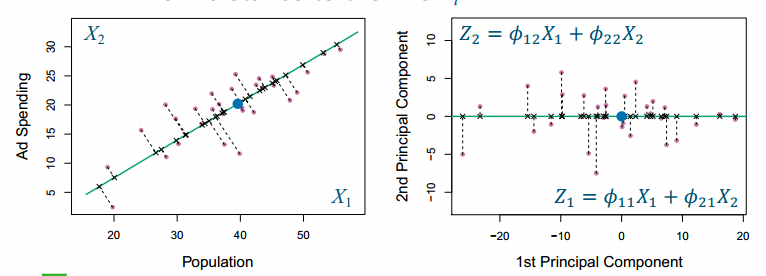
• Projecting points on a line Zi (principal component, PC): maximum variation along the line Zi数据在这个方向上的分布变化幅度最大,也就是minimum distance to the line Zi通过最大化方差来选择主成分方向，等价于通过最小化距离来选择低维子空间。
• Principal components are ordered: Z1 is the direction of most variation,Z2 is the direction of most variation perpendicular to Z1, Z3 is the direction of most variation perpendicular to Z1 and Z2

  Find the first principal component

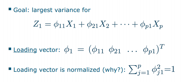
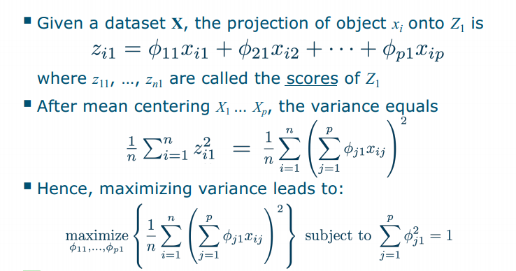  ![[a58dd338acf0a8836c37d61d757bd9f.png]] ![[da80bc059c23d325614c10cc5caef2e.png]] 通过使载荷向量的长度最大化(1)来最大化方差

  size does matter

• Scaling to unit standard deviation is useful if features have different ranges
• Scaling is essential if measured in different units,
• If units are the same, maybe we do not want to scale to unit variance as we may inflate noise这是因为单位方差假设所有特征的方差应该相等，但在这种情况下，这种假设可能不合适。

  biplot

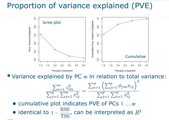
  PVE(proportion of variance explained)

![[a231610ce8f6af47eafbf207cd98180.png]] 就是那个loading vector就是PC的系数值， 同时也是pca.component_(如果在df才拟合的话)，也就是z

How to choose number of PCs?

• As few PCs as possible, retaining as much information as possible
• no clear solution: scree plot(PVE90%-95%); regard as tuning parameter, optimize by cross-validation; use additional information; visualization(2D,3D)

  Another interpretion of PCA

• Projecting points back into original space
• PCA minimizes reconstruction error

  Limitation and Solutions

• Linearity: kernel PCA (last week)
• Orthogonality:independent component analysis (ICA), maximizes independence of components

  Clustering vs. classification

• Classification:build predictors for categories based on an example dataset with labels
• Clustering:find ”natural” groups in data without using labels
• Classes and clusters do not necessarily coincide!
• Classes can consist of multiple clusters, clusters can combine classes ![[18d6fe7596d3687d334c898005a0ee5.png]]
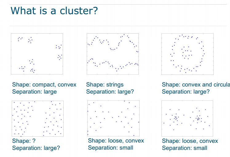
• Define what is “far apart” and “close together”: need a distance (or dissimilarity) measure to capture what we think is important for the grouping the choice for a certain distance measure is often the most important choice in clustering!
• Clustering is an ill-defined problem –there is no such thing as the objective clustering

  Hierarchical clustering

  ![[223220e0932c49db11e05bb4cce346f.png]]

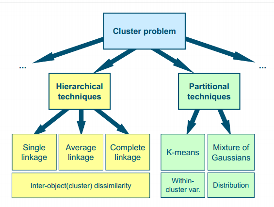
  Hierarchical clustering

• create dendrogram (tree) assuming clusters are nested
• bottom-up or agglomerative (as opposed to top-down, e.g. as in decision tree or K-means)
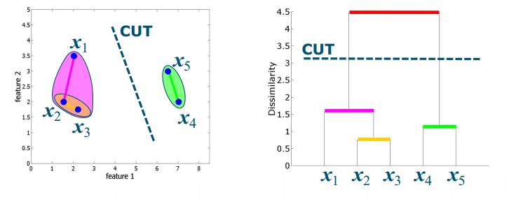
• Cutting the dendrogram(树状图) decides on number of clusters（簇） ![[4c86068c8ea033c8d2e2f7084e69b73.png]]

  Algorithm

• start: all objects of X in a separate cluster
• clustering: combine (fuse) the 2 clusters with the shortest distance in dissimilarity matrix D
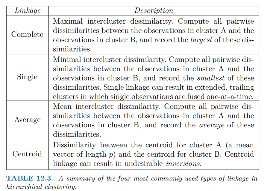
• distance between clusters is based on link type:
• single, complete, average, centroid, …
• repeat until only 1 cluster is left

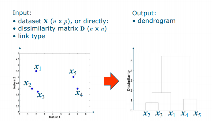
  Steps

• Step 1: Find the most similar pair of clusters: here x2 and x
• Step 2: Fuse x2 and x3 into a cluster [x2, x3]
• Step 3: Recompute D –what is the dissimilarity between [x2, x3] and the rest?
  1. single link: the smallest dissimilarity (nearest neighbor)
  2. complete link: the largest dissimilarity
  3. average link: the average dissimilarity
  4. centroid link: the dissimilarity to the cluster centroid ![[9adf1035b3bb7a85162f0636d433ad5.png]] ![[5ad171017b117bd03b6489f5cca65c5.png]]
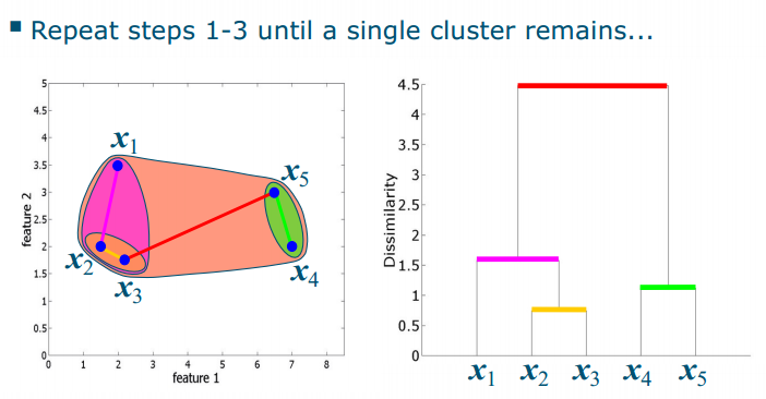
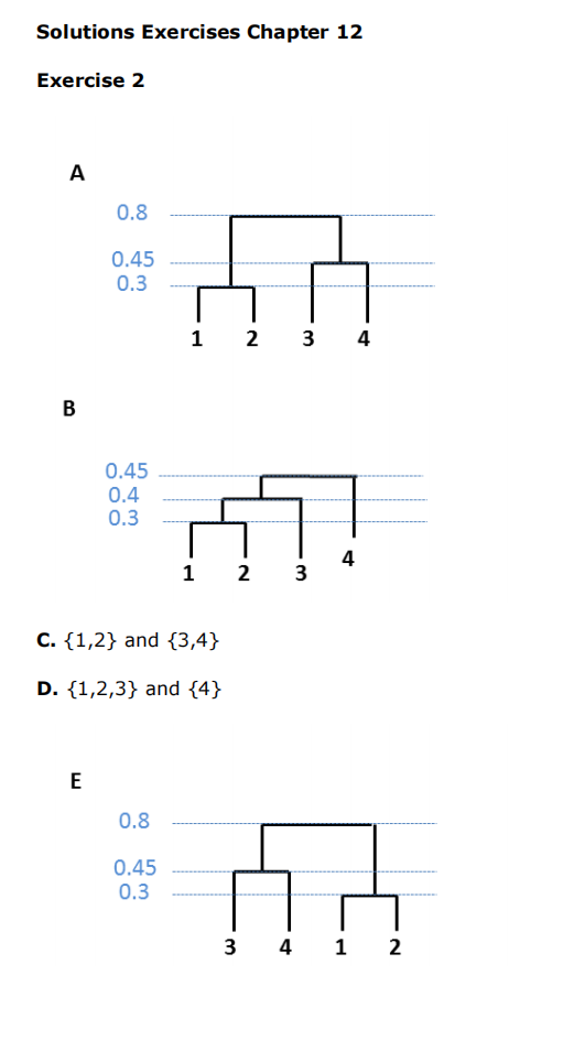
• Finally, cut the dendrogram to obtain clusters(Number of clusters: cut largest “gap” in tree (cf. elbow)) ![[b51d009bfa6c584f4d2b8f6d0aae2a7.png]] exercise ![[6c90858de0ca4ad2b5e4d8ae46ee40c.png]]![[bffcfda2516a3730c5b112f45aef77e.png]]

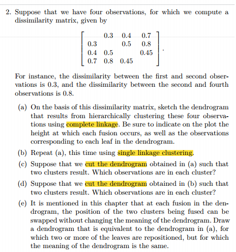
  Linkage

  No single best option:depends on data and intended use

• Average/centroid and complete linkage generally give more balanced trees
• Single linkage can find non-globular clusters, but is sensitive to outliers
• Centroid linkage can give inversions

  Scaling

• Depending on dissimilarity measure used, feature scaling can influence results (e.g. Euclidean distance) or not (e.g. correlation)
• When using Euclidean distance
  1. centering to mean zero to focus on trends instead of absolute value
  2. different measurement units may be a reason to scale to unit standard deviation

     Recap

• Unsupervised learning ● discover structure in only X, without a Y
• Dimensionality reduction: ● find low-dimensional representation that captures as much information as possible ● linear vs. nonlinear
• Principal component analysis: ● find orthogonal directions that maximize preserved variation or (equivalently) minimize reconstruction error ● scores, loadings, biplots
• Clustering: ● finding natural groups in data ● requires clustering algorithm and dissimilarity measure ● essentially subjective, no “proof”
• Hierarchical clustering: ● repeatedly fuse clusters, create dendrogram ● choice of linkage: single, complete, average, centroid ● cut dendrogram to find actual clusters